Bare-Metal Transformers: Cracking the Code on RMSNorm and Fused Kernels

Why modern LLMs dropped LayerNorm, how to compute the scaling math by hand, and the hardware-level trick that saves trillions of compute cycles.

Introduction: The Highway Bottleneck in Your GPU

Imagine you run an elite shipping warehouse. Your workers are incredibly fast at packaging items (this is your GPU’s computing units, or ALU). However, every time they package an item, they are forced to walk all the way across the facility to a slow, distant filing cabinet (High-Bandwidth Memory, or HBM) to write down an intermediate measurement, walk back, read it, and then finish the box.

No matter how fast your workers pack, your actual throughput is limited by the walking speed across the floor. This is the Memory Bandwidth Bottleneck, and it is the exact reason early Transformer architectures stalled.

In this deep dive, we break down Root Mean Square Normalization (RMSNorm)—the lean, mean stabilization layer that powers architectures like LLaMA, Mistral, and Gemma by turning a slow two-pass memory sweep into a single, blazing-fast pass.

At the end of this post, you’ll find a link to download an empty PDF workbook to trace this math yourself. Let’s solve it from scratch.

1. The “Why This Failed” Roadblock

Early Transformers relied heavily on standard LayerNorm. To stabilize training, LayerNorm forces activation vectors to maintain a zero-mean and unit-variance.

While mathematically clean, it creates a bare-metal nightmare: The Two-Pass Memory Sweep Problem.

\(LayerNorm: [Read Data] -> Calculate Mean -> [Save to HBM] -> [Re-read Data] -> Calculate Variance -> Normalize\)

Because the processor must calculate the mean first, it has to look at the entire vector, store that mean, and then read the exact same vector elements a second time to compute the variance. Moving these vectors back and forth between high-latency HBM and low-latency SRAM registers wastes precious clock cycles.

The Solution: RMSNorm

RMSNorm relies on a beautiful insight: Subtracting the mean (shift-invariance) doesn’t actually contribute to training stability. By dropping the mean-centering step completely, we scale activations strictly by their root mean square.

This collapses the math into a highly optimized, single-pass sweep. Data is read once, scaled inline, and pushed forward.

2. Core Mathematical Architecture

Instead of tracking both mean (μ) and variance (σ²), RMSNorm tracks a single scaling metric.

Given an activation vector x of dimension d:

\(1. \text{ Mean of Squares (MS)} = \frac{1}{d} \sum_{i=1}^{d} x_i^2\)

\(2. \text{ Root Mean Square (RMS)} = \sqrt{\text{MS} + \epsilon}\)

\(3. \text{ Normalized Vector Layer} = \frac{x_i}{\text{RMS}}\)

\(4. \text{ Final Scaled Output } (y_i) = \left( \frac{x_i}{\text{RMS}} \right) \cdot \gamma_i\)

Where γ (Gamma) is a learnable parameter vector initialized to ones, allowing the model to adaptively rescale dimensions during training.

3. Tensor Shape & Dimension Mapping Registry

Before the tensors hit the hardware, their structures must line up perfectly across our attention and normalization blocks:

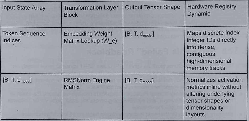
Notation: B = Batch Size; T = Sequence Token Length; d_model = Hidden Model Vector Dimension.

4. Pen-and-Paper Tracking Workspace (Fully Solved)

Let’s trace a concrete example. Assume an input token passes through our embedding layer and yields a dense activation state vector:

x = [2, -2, 4, 0]

The layer dimension is d = 4. Our learnable scaling parameter configuration is initialized to γ= [0.5, 1.0, 2.0, 1.5]. For numerical stability, let’s assume ε = 0.

Step 4.1: Compute Element-wise Squares

Square each independent coordinate within the activation array vector:

• x₁² = 2² = [ 4 ]

• x₂² = (-2)² = [ 4 ]

• x₃² = 4² = [ 16 ]

• x₄² = 0² = [ 0 ]

Step 4.2: Compute Mean of Squares & RMS

Sum your squared metrics, calculate the dimensional average, and resolve the global scale factor:

• Sum of Squares = 4 + 4 + 16 + 0 = [ 24 ]

• Mean of Squares (Divide Sum by d=4) = 24 / 4 = [ 6 ]

• Root Mean Square (RMS = √6) ≈ [ 2.4495 ]

What is Epsilon (ε)? Epsilon is a tiny safety value (e.g., 10^-8) added inside the square root. If our input vector was completely dead ([0, 0, 0, 0]), our RMS would be 0. In Step 4.3, we would divide by zero, crashing our training run with NaN errors. Epsilon prevents this hardware crash.

Step 4.3: Calculate Normalized Activation Shifts

Divide each original input element by your calculated RMS scaling factor ( ≈ 2.4495):

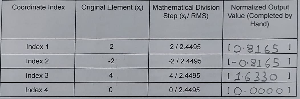
Step 4.4: Apply Learnable Parameter Gamma Scaling

Multiply each normalized vector element by its corresponding index position weight in the γ layer to find the final normalized model values (y_i = Normalized_i x γ _i):

• y₁ = 0.8165 x 0.5 = [ 0.4082 ]

• y₂ = -0.8165 x 1.0 = [ -0.8165 ]

• y₃ = 1.6330 x 2.0 = [ 3.2660 ]

• y₄ = 0.0000 x 1.5 = [ 0.0000 ]

5. Architectural Layout: Hardware-Aware Data Flow

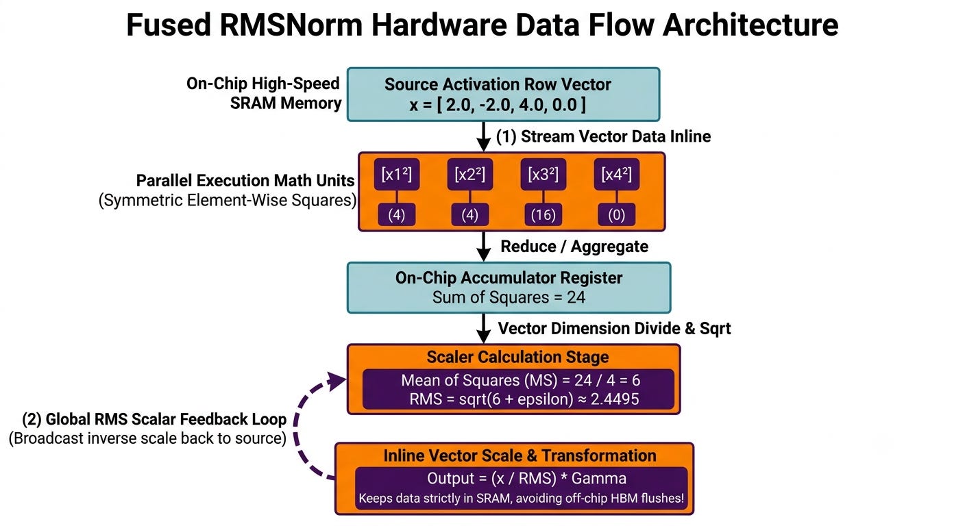
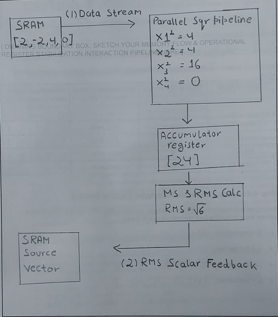
To understand why this is fast, we have to look at the silicon level. Instead of pushing data back to off-chip memory, a highly optimized fused kernel keeps everything local inside low-latency registers (SRAM).

Here is how data streams through an accelerator chip during a single-pass RMSNorm block:

Hand-Drawn RMS Architecture Diagram for Workbook

6. Bare-Metal Memory Insights & Fused Kernel Implementation

In high-performance deep learning libraries (like FlashAttention or vLLM), execution efficiency is won by avoiding memory access roundtrips. Writing an un-fused operation forces a processor to write intermediate normalized states back to high-latency HBM before executing subsequent scaling tasks.

Fusing the calculations into a single hardware sweep keeps data entirely inside fast on-chip registers. Here is a clean python verification matching our hand-calculated tracking:

Python

import math

def first_principles_rmsnorm(x, gamma, epsilon=1e-8):
    # Element dimension calculation
    d = len(x)
    
    # Step 1: Compute element-wise squares and sum
    sum_of_squares = sum([element ** 2 for element in x])
    
    # Step 2: Calculate Mean of Squares
    mean_of_squares = sum_of_squares / d
    
    # Step 3: Resolve Root Mean Square scaling factor
    rms = math.sqrt(mean_of_squares + epsilon)
    
    # Step 4: Map normalized elements and apply gamma scaling inline
    output_vector = [(element / rms) * gamma[i] for i, element in enumerate(x)]
    
    return output_vector

# Machine Execution Verification Step
input_activations = [2.0, -2.0, 4.0, 0.0]
gamma_parameters = [0.5, 1.0, 2.0, 1.5]

resulting_tensor = first_principles_rmsnorm(input_activations, gamma_parameters)
print(f"Machine Output: {resulting_tensor}")
# Machine Output: [0.4082482904638631, -0.8164965809277261, 3.2659863237109043, 0.0]

Notice how closely the python calculations match our manual workspace limits. By forcing loops to execute strictly along individual rows of data, modern GPU architectures can avoid pointer redirection entirely. This prevents pipeline stalls across deep frontier clusters.

7. Grab the Empty Workbook PDF

Want to cement these concepts in your muscle memory? We’ve prepared a clean, unfilled PDF version of this workbook layout containing the structural shapes, empty evaluation brackets, and drawing boxes. Print it out, step away from the screen, and trace the activations with a pencil.

👉 [Download the Empty LLM Workbook 2: RMSNorm PDF Workspace Here]

What are your thoughts on kernel fusion or hardware acceleration constraints? Let’s discuss in the comments below!

7. First-Principles Reference Log

This tracking framework structures the foundational design patterns introduced across the modern large language model optimization architecture:

• Zhang, B., & Sennrich, R. (2019). Root Mean Square Layer Normalization. arXiv preprint arXiv:1910.07467.

• Touvron, H., et al. (2023). LLaMA: Open and Efficient Foundation Language Models. arXiv preprint arXiv:2302.13971.

• Karpathy, A. (2024). Let’s build GPT from scratch from first principles. Educational Deep Dive Architecture Track.