Extrapolating to Infinity — Attention with Linear Biases (ALiBi) by Hand
Why modern LLMs abandon absolute positions, how to calculate distance penalties by hand, and the bare-metal hardware reasons why context windows break.

If you’ve been following the frontier of LLM development, you know that the biggest architectural battle right now is being fought over context length. We want models that can process entire code repositories, legal libraries, or medical history scrolls without breaking a sweat.
But traditional Transformers hit a hard wall. If you train a standard model on a 2,048-token context window and suddenly feed it 5,000 tokens at inference time, it goes completely haywire. It starts outputting absolute gibberish. This is known as the Extrapolation Crisis.
Today, we are going to demystify ALiBi (Attention with Linear Biases)—a remarkably elegant architectural “hack” that solves this problem entirely by transforming position tracking into a simple, static distance tax.
We’ve attached an [Empty Practice Workbook PDF] at the bottom of this post so you can print it out and trace the math with a pencil. In this post, we’ll step through the complete, fully solved workbook together.
Let’s dive in.
The Architectural Roadblock: Why Space Encodings Fail
Traditional positional methods try to give tokens coordinate identities early on.
Absolute Position Embeddings add a static coordinate vector to the token vectors right at the entrance gate.
RoPE (Rotary Position Embeddings) rotate the Query and Key vectors in complex vector spaces based on their exact sequence indices (m and n).
The structural flaw? The model’s weights become highly dependent on the absolute numbers or exact rotation angles encountered during training. When word 4,000 shows up at runtime, the model sees geometric configurations it has literally never witnessed before. The internal math destabilizes.
Enter ALiBi: Distance as a Tax on Attention
ALiBi completely flips the paradigm. It says: Stop trying to invent complex geometric coordinates. Let’s look at a fundamental property of human language: The further away two words are from each other, the less they should care about each other.
Instead of changing the vectors before they calculate their relationship, ALiBi lets the words compute their raw similarity scores (QKT) completely oblivious to position. Once those raw scores are calculated, we step in and charge a relative distance tax.
Because this “tax” is a simple subtraction based on how far apart two tokens are, the formula never changes, whether a sentence is 10 words long or 10,000 words long.
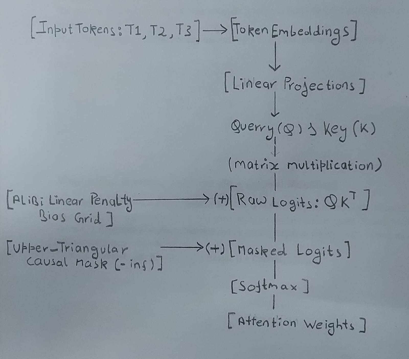
The Architectural Blueprint
Before we touch the numbers, look at how clean this topology is compared to RoPE or Absolute Embeddings. Notice that the position block completely avoids the input token pathway and modifies the system at the matrix multiplication layer:
SECTION 2: Pen-and-Paper Math Tracker (Solved)
Let’s play the role of the GPU attention engine and calculate a 3-token sequence tracking by hand.
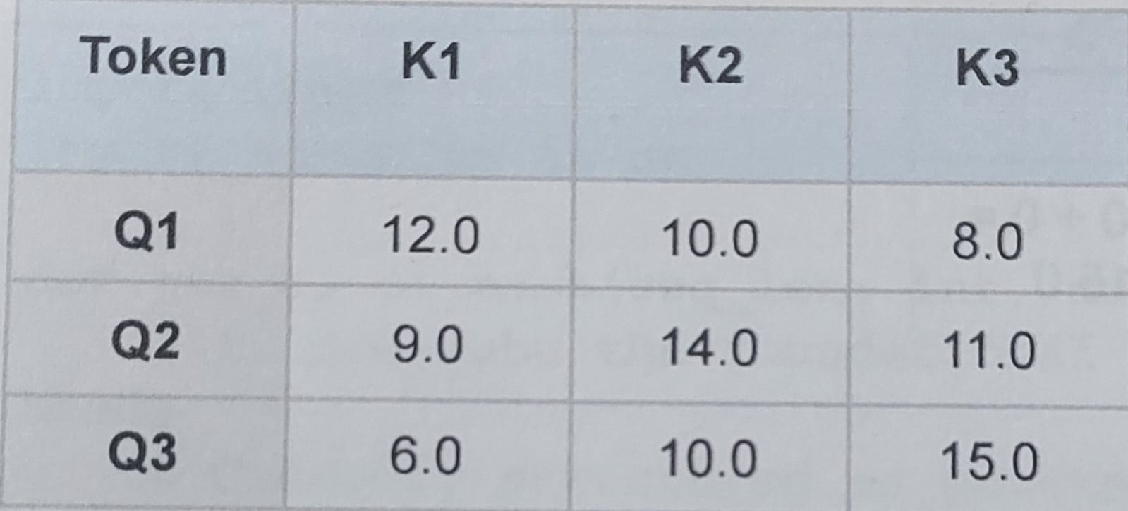
The Input State
We begin with a pre-calculated, raw dot-product logit matrix (QKT) matching the dimensions [3 x 3]:
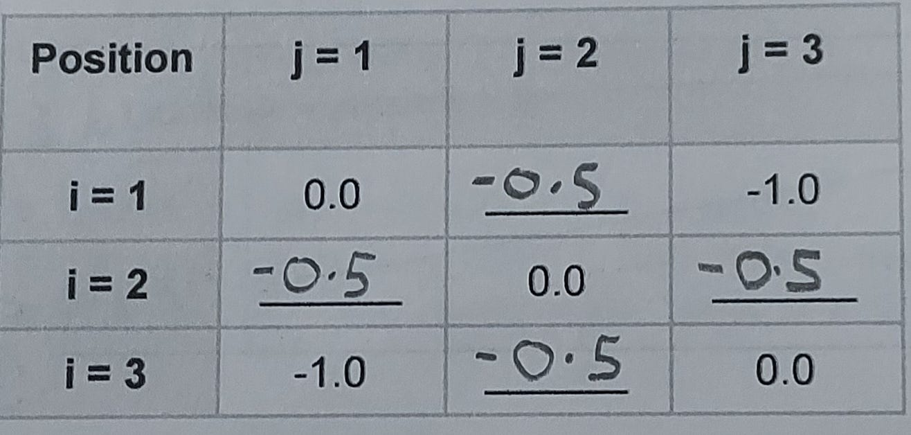
Step 1: Slope Matrix Construction
ALiBi multiplies a relative distance matrix by a head-specific slope factor, m. For this specific attention head, our assigned slope factor is m = 0.5.
The relative distance penalty formula between query position i and key position j is:
The Hand-Calculations:
The Completed Bias Grid (m = 0.5):
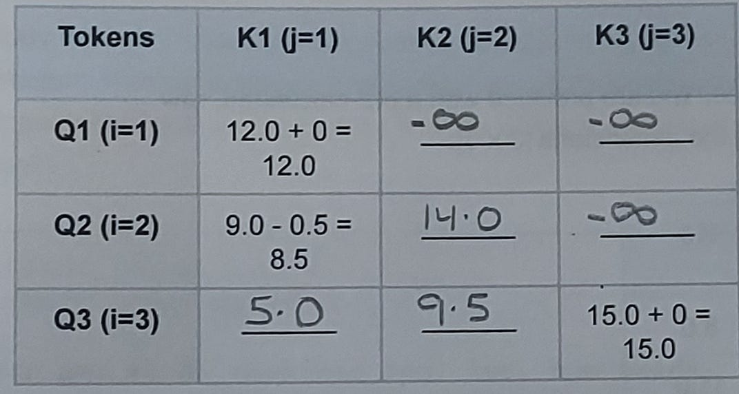
Step 2: The Masking Pass (ALiBi + Causal Masking)
Now, we must combine our raw QKT matrix with the Bias Grid we just calculated. Additionally, because this is an auto-regressive decoder model, we must apply a standard causal mask. Future tokens (where j > i) must be completely blanked out by adding negative infinity (-inf), forcing their final softmax probabilities to 0.
The Hand-Calculations:
Row 1 (i=1): Tokens K2 and K3 are in the future (j > i). They are blocked —>
-inf.Row 2 (i=2): K3 is in the future —>
-inf. K2 is distance 0: 14.0 + 0.0 = 14.0.Row 3 (i=3): No future tokens.
For K1: 6.0 - 1.0 =
5.0For K2: 10.0 - 0.5 =
9.5
The Completed Masking Pass Matrix:
SECTION 3: Visual Workspace & Decay Profile
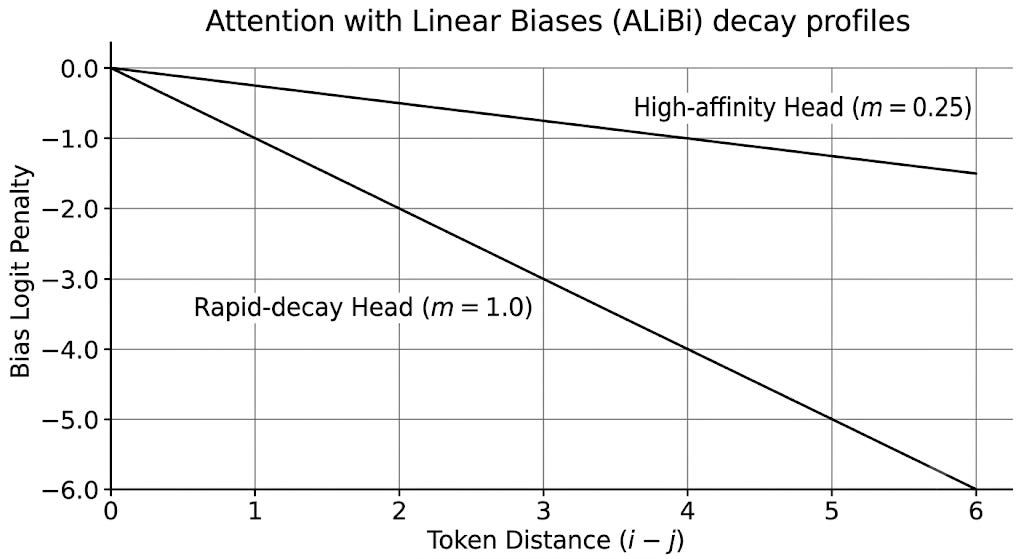
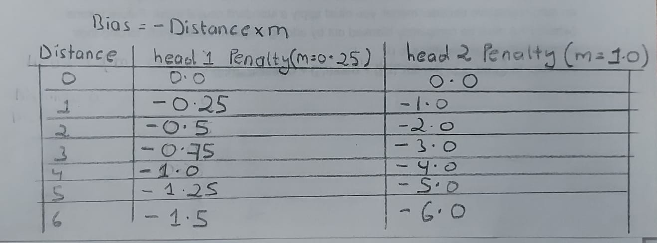
Different attention heads are assigned different slope values (m), usually scaling as powers of 2 (e.g., 2-8/n). This creates a diverse memory profile across the network.
If you plot a High-Affinity Head (m = 0.25) alongside a Rapid-Decay Head (m = 1.0) out to a token distance of 6, you can visually see how the network balances short-range and long-range context:
SECTION 4: Bare-Metal Code Implementation
Here is a zero-dependency PyTorch implementation of this process. Notice the absolute absence of complex index-tracking matrices or trigonometric coordinate math:
Python
import torch
import torch.nn as nn

def get_alibi_mask(seq_len: int, num_heads: int) -> torch.Tensor:
    # 1. Generate the foundational slope arrays for all attention heads
    # Commonly structured as geometric sequences based on powers of 2
    start_slope = 2 ** (-8 / num_heads)
    slopes = torch.pow(start_slope, torch.arange(1, num_heads + 1))

    # 2. Build the basic relative distance coordinate layout
    # Shape: [seq_len, seq_len]
    context_position = torch.arange(seq_len).unsqueeze(1)
    memory_position = torch.arange(seq_len).unsqueeze(0)
    relative_distance = torch.abs(context_position - memory_position)

    # 3. Project the distance matrix across the head dimension
    # Shape: [num_heads, seq_len, seq_len]
    alibi_bias = relative_distance.unsqueeze(0) * -slopes.unsqueeze(1).unsqueeze(2)
    return alibi_bias

# Architecture Verification:
# If you run get_alibi_mask(seq_len=3, num_heads=1) and set the slope to 0.5,
# the resulting tensor matches our hand-calculated Section 2 Bias Grid perfectly!
SECTION 5: Hardware Connection Notes
Why does this matter under the hood? In massive production inference clusters, memory bandwidth is the primary bottleneck.
When using traditional absolute lookup arrays or complex Rotary transforms (RoPE), the GPU must continually pull positional index trackers or compute transcendental mathematical steps inside high-bandwidth memory (HBM) arrays before loading them into active SRAM registers.
ALiBi eliminates this hardware block. Because the linear bias structure is perfectly static and depends strictly on the row and column shapes of the current generation slice, it can be fused directly into custom FlashAttention compute kernels.
The system avoids extra intermediate allocations entirely. The GPU registers remain wide open for pure, uninterrupted matrix multiplications—making auto-regressive text streaming incredibly fast.
📥 Download the Empty Workspace PDF
Want to trace this math yourself from a clean slate? Download the empty pen-and-paper workbook below and see how long context tracking works without looking at a computer screen:
👉 [Link to Download: Attention Workbook 6 — Empty Practice Template (PDF)]
What are your thoughts on ALiBi versus newer hybrid attention schemas? Let’s talk in the comments below!